This post continues from Part One, where we walked through how to securely onboard a production-scale fleet of IoT devices streaming telemetry data to your Google Cloud environment via IoT Core and Pub/Sub, and Part Two, where that data was moved seamlessly from Pub/Sub to BigQuery via Dataflow, then visualized with Data Studio.

If you have been following along with my previous articles, you have enjoyed setting up temperature sensors throughout your home and watched as their live-streamed data flows seamlessly into GCP, ultimately landing in Google’s data warehouse service BigQuery. What now? How can we make practical use of this data?

To answer those questions, I would like to demo a working example using one of BigQuery’s most unique and powerful features: BigQuery ML.

If you have not followed along with the previous articles, fear not! I have made my dataset available on Kaggle; feel free to use that as you follow along.

BigQuery ML Overview

Unlike other data warehouse services, machine learning training and deployment is built right into BigQuery. Both training and deployment are performed with SQL-like commands that are simple to construct.

With only a few lines of SQL-esque code, you can specify the type of model to create, such as models based on logistic or linear regression, k-means clustering, deep neural networks, and so on. Or, you can leave it up to Google by creating an AutoML Tables model, as we will do in this article. Most models require no specifications beyond providing the label and feature columns.

Before we can jump into the specifics of how to initiate ML training within BigQuery, we must first determine how raw temperature data can be used as a predictive model and what data transformations need to take place prior to model construction. Machine learning is 90% data preparation, after all.

Machine Learning Goal and Methodology

At the time that I am writing this article (Feb 2021), it is a chilly 48 degrees Fahrenheit in Oregon. The heater is chugging along, keeping me nice and toasty while I work, but every now and then I would like to leave a window open to refresh the air in the house — especially since I have a nine-week-old Corgi who isn’t fully potty trained yet!

What I would like to do is be able to open a window, and if it remains open for too long of a period of time have GCP remind me that it’s open. Don’t want to waste too much electricity! If possible, I would like the temperature sensors scattered throughout the main living space of my home to also tell me which specific window to close.

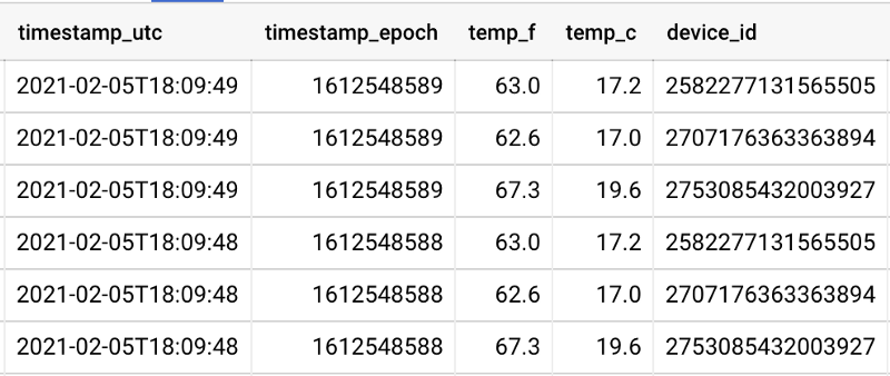
There are three sensors streaming temperature telemetry data into my GCP project, and they are each positioned near their own window in the main living room in my home.

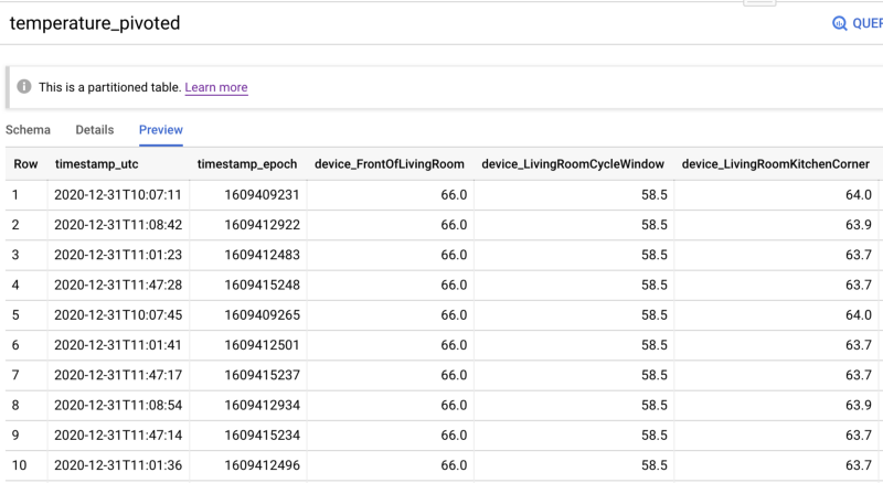
Two sensors are very close to their own windows, while a third is about 8 feet away from its nearest window. You can see sensor proximity to the windows reflected in the data, where one sensor (device_id) reports values several degrees warmer than the other two:

In order to build a machine learning model that can identify when a specific window is open, we need to engage in a few data transform steps to yield the end table ready for ML model training. Training a model requires:

1. Tracking time frames when a window is open. I manually entered “window #1/2/3 is open” start and stop times in Excel. Non-tracked time frames are assumed to have closed windows. This table will eventually be converted to CSV and loaded as a BigQuery table.
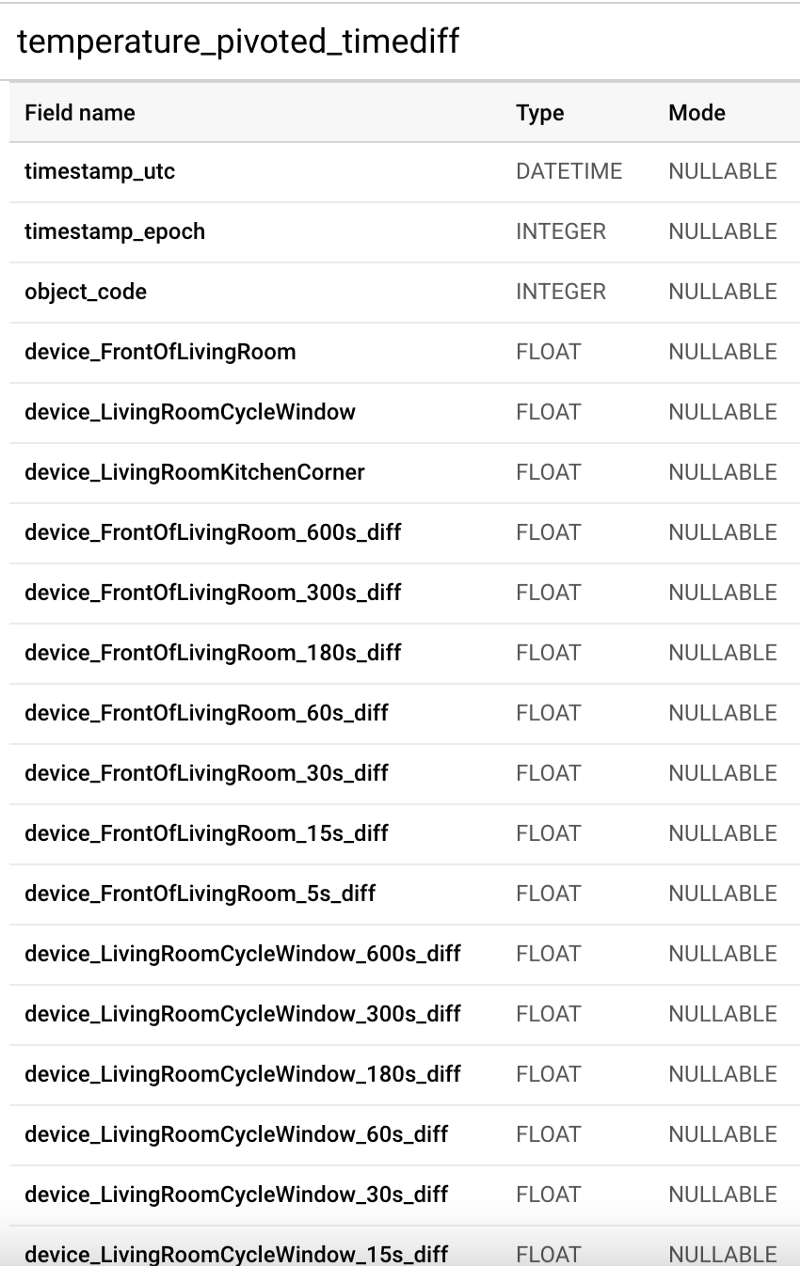
2. Transforming the raw streaming temperature data table, where each row contains a sensor-specific temperature value for a specific second, into a pivoted table where each individual second has its own dedicated row of data. Each per-second row will possess columns storing each device’s temperature for that moment, as well as columns showing the difference between a sensor’s current value and its value x number of seconds ago. The purpose here is to track each sensor’s current temperature value, as well as how much that value has changed from some time interval in the past: 10 minutes ago, 5 minutes, 3 minutes, 1 minute, and so on down to 5 seconds ago. These columns will act as excellent predictive features.
3. The BQ table defining time frames when windows are open and closed should be merged with the pivoted temperature table, providing us with a final table that contains our predictive temperature feature columns and an open window / all windows closed label column.

Let’s quickly walk through how to perform each of these steps.

Tracking Open Window Timeframes and Loading Them into BigQuery

As I opened one of three windows in my home, I manually tracked the precise moment a specific window was opened in an Excel table:

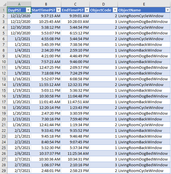
Note that ObjectCode values one through three each represent a specific window, while an unspecified value of zero will be used later to represent all windows that are closed.

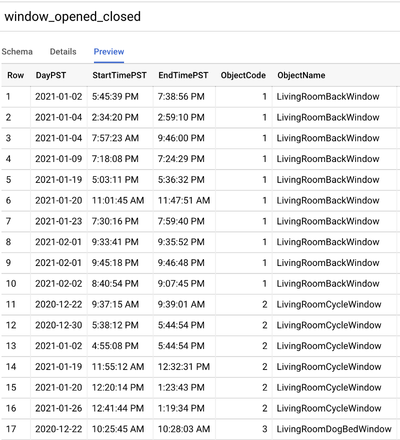
After gathering what I felt was enough data points over the course of 1.5 months, I exported this to a CSV, uploaded that CSV to a Cloud Storage (GCS) bucket, and then ran the following command to create a new BigQuery table from this with the schema auto-detected:

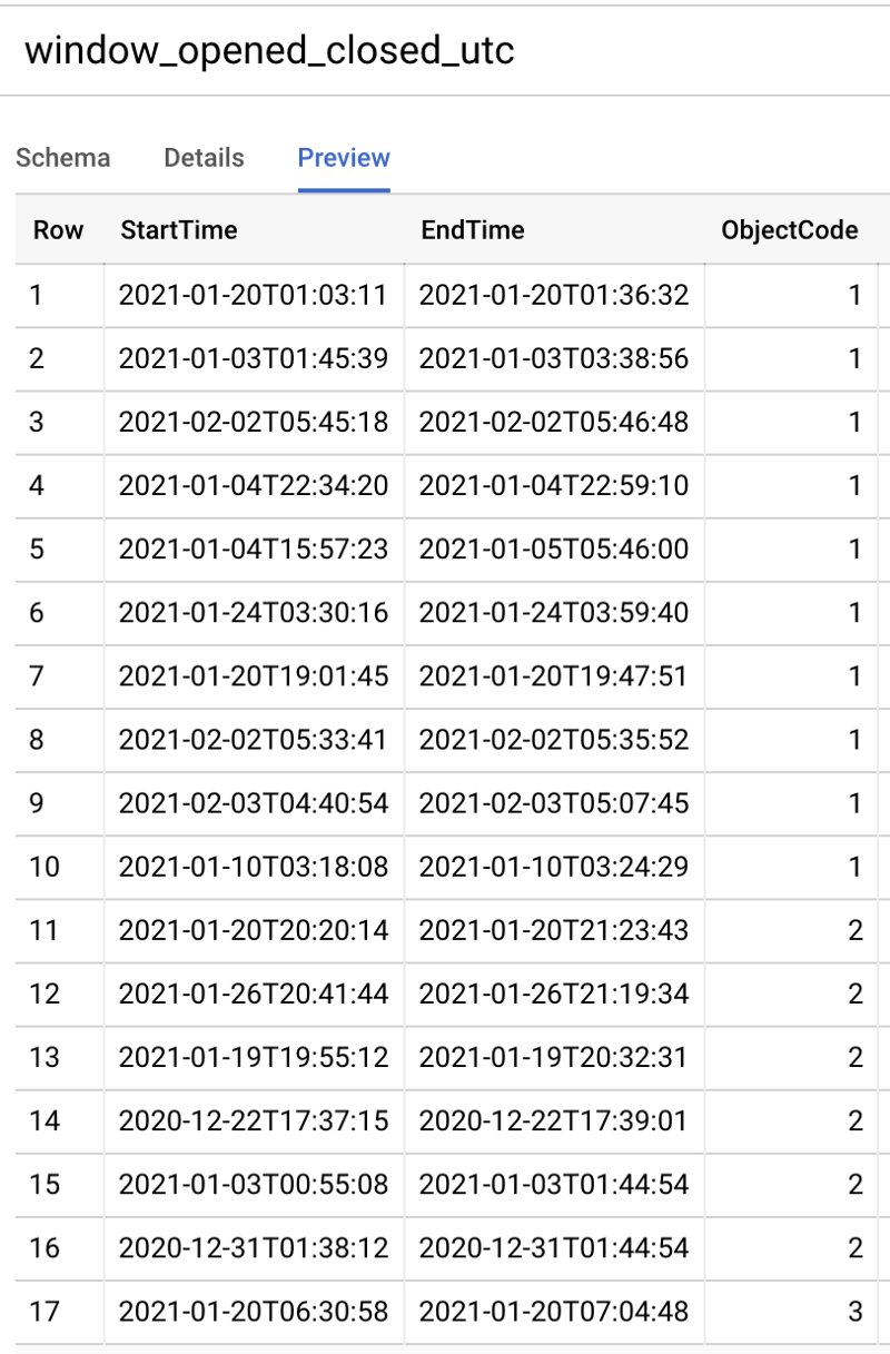
Since the streaming data is:

1. Stored in UTC rather than the PST value I manually recorded, and
2. Storing datetime values rather than separate date and timestamp values I manually recorded

I ran the following SQL command to convert open window start and end time points to universal time standard datetimes:

Before we join these window open/closed states to temp time points, we must first pivot our raw data table so that all sensor values for a given second are present in one row.

Side-note: If you are working with raw temperature data from my Kaggle dataset rather than your own streaming data, use the following to import that CSV into your project before moving on:

Datetime-Pivoted Temperature Table Creation

Pivoting the raw per-second, per-sensor temperature data table into per-second rows with all sensor values present can be done with the following SQL. Note that in this query, I am also excluding rows of data where one or more sensors failed to record a value. There were many instances where the power went out — my entire house for an hour on Christmas Day, Roomba bumping into a sensor power cord, Maple knocking a sensor over…expect the unexpected!

You might be able to get away with imputing reasonable defaults for these null values (for example, with an average of the values from that sensor over the past 60s). However, in my dataset there are ~10.5M rows of raw data, which is more than enough to train the model. It is likely better to exclude rows with null values from model training altogether rather than attempt a guesstimation for reasonable default values.

We are almost ready to begin training our model! We need only to create one more table which contains the following:

1. A merging of time points to known open window states. All time points missing an open window state receive a closed state value by default.
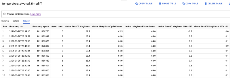
2. Creation of retrospective temperature value columns. While knowing a device’s temp for a given second is useful, it would be more useful to enable a comparison of the current value against various past time points.

To achieve these goals, I run one final SQL statement creating the final BigQuery table which will act as input for our machine learning training process. I want to note that there is a much faster, although considerably more expensive, means for obtaining these retrospective values, but we’ll talk more about that later.

With this final table, we at last have everything we need to begin training a BigQuery ML model.

BigQuery ML Training

The following four lines of SQL-like code tell BigQuery to:

• Train an ML model using Google’s AutoML Tables algorithm. If this takes longer than 24 hours, cut the training short and work with the best model generated thus far.
• Use “object_code” (window open/closed state) as the column to predict.
• All other columns are to be used as features except the datetimes.

Run this, wait for it to complete, and that is it. Seriously!

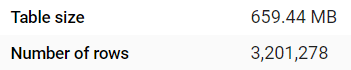
Given that the pivoted dataset is quite large at 25 columns and ~3.2M rows, or about 80M cells of data, and knowing that AutoML repeatedly trains and evaluates a multitude of computationally intensive deep neural networks, this will take some time to complete.

BigQuery ML Training: Cost Warning

At the time of writing this article, BigQuery’s AutoML feature is charged at “$5.00 per TB, plus AI Platform training cost”. You might expect this to be a fairly cheap training operation given that the pivoted table we are training on is 659 MBs in size:

However, AutoML creates and then scans many temporary datasets as part of its DNN training process. When the 24 hour-limited model at last finished generating, it had processed (and billed!) more than 89 TBs of data:

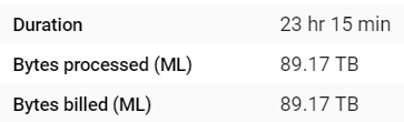
This comes out to a cost of $445.85, not including the obfuscated processing charges incurred behind the scenes by BigQuery using the AI Platform for its training which brought the total cost up to around $500.

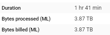
If you intend to test BQ ML without spending much money, be cautious around how many hours of training time you budget for. Changing BUDGET_HOURS from 24.0 to 1.0 hours yields a model that finishes in 1h41m and only processed 3.87 TBs, or roughly $19.35 (plus hidden training compute costs):

BigQuery ML Training Results

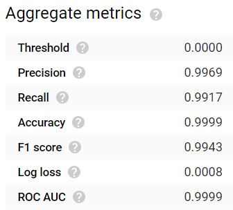
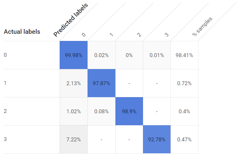
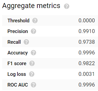
After waiting 24 hours, the model finished generating. The results are quite impressive! Common evaluation metrics such as accuracy, precision, recall, F1 score, and ROC AUC all yield values ≥0.99:

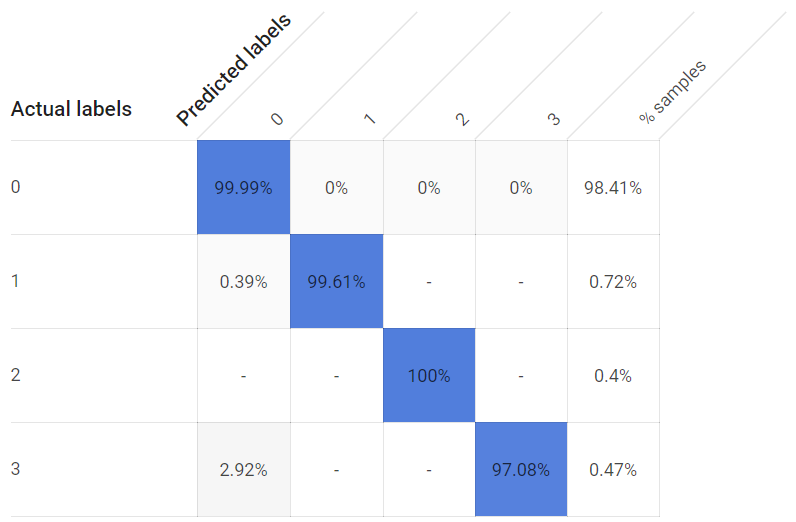
Despite exceptionally unbalanced representation among the label classes — windows remain in the closed state far more often than in the open state as I don’t want to raise my electric bill too much — each open window state nonetheless possesses exceptionally high true positive rates. Even the third window, whose closest sensor is about eight feet away rather than inches away, managed to yield a true positive detection rate of >97%:

Generating a model with a one hour cutoff produces a usable model, although the TP rates for individual classes are lower, and substantially so for the third window with its more distant temperature sensor:

It’s pretty cool how easy it is to build a functional ML model using BQ…but is it useful? Is the 24h model truly effective? How can we get predictions using this model?

Deploying the model within BigQuery and yielding predictions is as simple as running two lines of SQL code after you format your raw data back into a pivoted table format.

BigQuery ML Deployment and Predictions

The following SQL formats raw streaming temps into the pivoted table format, then feeds this into the BQ ML model for predictions. Ultimately, the query returns open/closed window predictions for the past 600 seconds.

If this query were run from within a Cloud Function (a serverless code service) every 60 seconds using Cloud Scheduler (a cron job service), and if ≥95% of predictions over the past 10 minutes were called in a non-zero state, you could set that Cloud Function up to immediately send an e-mail or a text message mentioning that x window has been open for too long and needs to be closed. Such an alerting system allows for a brief opening of the window, and notification when it is left open for too long.

While the following may seem like a lot of code to get predictions, all but the final few lines are simply data prep, the gathering of raw data together into the proper pivoted table format for use as model input.

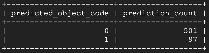
Let’s see how this model performs when all windows are closed:

Nine seconds later, the majority of which was spent on data table pivoting rather than model prediction:

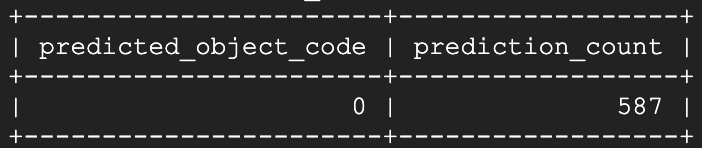
Not bad at all! It looks like we’re missing the most recent 13 live-streaming seconds of temperature values from one or more devices, and the remaining 587 seconds are all correctly identified as in the closed state.

After opening window #1 up and waiting about 15 seconds, I re-ran the prediction script:

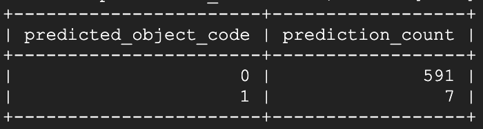
Voila! Within a few seconds after opening, the model has begun to identify that specific window as open. Running the prediction script again about a minute and a half later:

We can see that the open state is being clearly and continually identified!

As time passes, the open state will outnumber the closed state predictions over a 10 minute time window, until eventually it dominates the windowed prediction count. At that point, a Cloud Function could then be written which takes action and issues a notification to myself to close the dang window!

Email Alerting with a Cloud Function

Unfortunately, Google Cloud does not offer SMS or email services, instead redirecting customers to use third party companies. Showcasing e-mail or SMS through a Cloud Function with an external service would be both pricey and lengthen this already long article, so we’ll cut the tutorial short here.

If you do have an email service available to you, a script similar to the following should work well for alerting via a Python Cloud Function:

Rapid Retrieval of Retrospective Temperatures with a BigTable External Table

A good chunk of the pivoted table data transformation SQL is dedicated to retrieving “current minus past temperature” values for each individual second. Performing these backwards-looking INNER JOINs entirely with BigQuery, while doable, is not going to be highly performant at scale. BigQuery is best optimized for massive-scale analytics on one table. As with all data warehouses, it cannot support indexes as a result of enabling petabyte-scale storage and analytics, and this makes JOIN operations very computationally intensive and something to be avoided whenever possible.

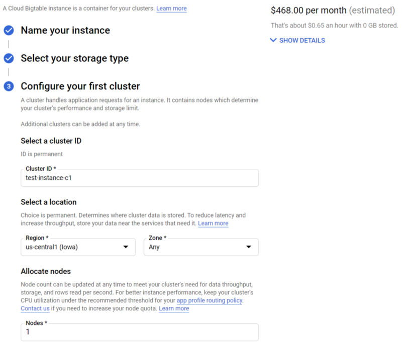
You might want to consider setting up a BigTable instance, Google Cloud’s massively scalable NoSQL database service that offers single digit millisecond response times for individual row queries, and duplicating storage of your raw temperature data within this service. Within BigQuery, you can set up a BigTable instance as an external table, then perform queries against this table as if it were a BigQuery table.

If you were to set up a second Dataflow job that moves your IoT data hitting a PubSub Subscription into BigTable, making sure to use a primary key combining deviceId and datetime, you would then be able to retrieve individual time points for a particular device and time point much faster than BQ SQL could when pulling entirely from native BigQuery tables.

With this approach, you would then update your pivoted table generation SQL to INNER JOIN to the BigTable external table using a device-datetime combo as the JOIN ON key.

This workflow should in theory be more scalable and highly performant, but it will also be considerably more expensive. Even a ‘cheap’ single node instance for development testing will run you $468 / month in us-central1. You should nonetheless try implementing this approach if you intend to deploy IoT operations at scale.

Conclusion

Congratulations for having stuck with this deep-dive into IoT and ML on GCP. I hope this has been instructional and helped accelerate you on your journey into ingesting, analyzing, and making real use of large-scale datasets in the cloud, utilizing as many fully-managed, auto-scaling, serverless services as are available in order to minimize time spent stressing over cluster uptime and maximize time spent getting meaningful work done.

As a reward for you patience and perseverance, the least I can do is offer up one final cute puppy photo!